Marketing Mix Modeling MMM (Part 3 of 3)

MMM assists marketers in optimizing future spends and maximizing effectiveness (i.e. it establishes which mediums are working better than others). Then, budget allocation is done, by shifting money from low ROI mediums to high ROI mediums, thus maximizing sales while keeping the budget constant.

Types of MMM

MMM can be built using regression methods and the most common regression techniques used are:

• Linear regression ($latex y =\beta_{1} + \beta_{2}X_{2} + … +  \beta_{k}X_{k} + \epsilon $); and
• Multiplicative regression

We can construct a regression equation that considers the proportion of investments in different marketing channels and develop an algorithm to maximize revenues.

Here, we will focus particularly on multiplicative regression models for MMM as they can manage increased complexity of marketing variables by fitting a flexible spline to data, instead of a straight line (i.e. the linear regression method does not perform well on large amounts of data as it is sensitive to outliers, multicollinearity, and cross-correlation). This gives more flexibility to incorporate as well as capture complex aspects like interactions and synergies within and between media groups, carryover effects of advertising, and diminishing returns of media (described by an S-shaped curve).

The two kinds of multiplicative regression models are:

• Semi-logarithmic models
• Logarithmic models

Semi-logarithmic models

In Log-Linear models, the exponents of independent variables are multiplied.

This can also be rewritten as:

Logarithmic transformation of the target variable linearizes the model form, which in turn can be estimated as an additive model. The dependent variable is logarithmic transformed; this is the only difference between additive models and semi-logarithmic models.

In Log-Linear models, the coefficients β are interpreted as the % change in business outcome (sales) for a unit change in the independent variables (e.g. pricing, distribution, media, discounts, seasonality, promotion, etc.).

Logarithmic Models

In Log-Log models, independent variables are also subjected to logarithmic transformation in addition to the target variable.

Rewriting the model in linear form:

The main difference between Log-Linear and Log-Log models lies in the interpretation of response coefficients. In Log-Log models, the coefficients β are interpreted as the % change in business outcome (sales) in response to a 1% change in the independent variable:

This implies constant elasticity of the target variable with respect to the explanatory variables. In Log-Linear models, elasticity cannot be directly estimated but can be calculated from the coefficient as βX for every time period. It increases in absolute value with the explanatory variable.

Case Study

We can understand the concept of MMM more effectively with an example. Consider Product ABC from a leading retailer. Marketing data for the product is available for October to December 2017 (table below).

*GRP (Gross Rating Point) is a measure of the size of an advertising campaign by a specific medium or schedule.

Question: What is the incremental lift in Sales (dependent variable) when TV GRPs are increased by 20% from the current level of 459 GRPs and discounts are increased by 10% from the current level of 9.28%?

Answer:

1. The objective is to maximize the target variable (sales). Since TV GRPs and discounts are the variables to be optimized, constraints are applied to these variables.
   • Weekly maximum for TV GRPs will be decided by the sigmoid curve (based on saturation point). Total TV GRPs is set at 20% from current levels.
   • Weekly maximum for discounts is set based on historic values. Average discounts is set at 10% from current levels.
2. The following table lists the current levels and constraints for TV GRP and discounts:

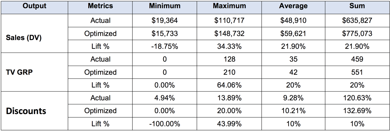
3. The data summary for the target variable and optimized variables are as follows:

4. The business recommendations, based on optimization results are as follows:
   • On increasing TV GRPs by 20% and Discounts by 10%, a Sales increase of 21.90% is achieved upon effective distribution.
   • More TV GRPs are spent during the holiday period (Nov-Dec) for effective sales
   • High levels of discounts are maintained during the holiday period with no discounts in other periods

Conclusion

Marketing mix modeling techniques can minimize much of the risk associated with new product launches or expansions. They are a key driver for business strategy and can improve the profitability of a company’s marketing initiatives. With this in mind, you can get started on developing a watertight marketing mix model that can maximise performance and sales of a new product.

Jason Oh is a Senior Consultant, Strategy & Customer at EY with project experiences in commercial due diligence and corporate strategy planning. Previously, he was a Management Consultant at Novantas with a focus on the financial services sector, where he advised on pricing, marketing, channel distribution, digital transformation and due diligence.

Image: Pexels

🔴 Interested in consulting?